Antenna Analysis from Ham Radio to PCBs
Comments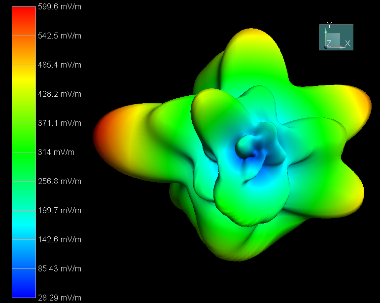
Has anyone else ever thought about why so many engineers are also active amateur radio operators? My theory is that there's just so much passion for the science and practical use of these complex electronic systems! We enjoy the problems, challenges and solutions so much that we want to find other ways outside of work to find those same experiences. In this case, I've got a story that starts with some amateur radio equipment but comes full-circle to address an extremely common design issue. Specifically, we'll look at the Arrow OSJ antenna performance as well as the characteristics of a printed circuit board antenna.
The Attempted QSO
This all begins with a new radio. I recently installed the FTM-3200DR1, a 2m-band, 65W transceiver with Yaesu's digital C4FM modulation. One of the first things I wanted to try with this radio was a direct, simplex QSO 2 with a friend who is about 16 miles away as the crow flies. Unfortunately for propagation, we've got a decent amount of hilly terrain up here in the Skylands region of New Jersey in addition to this being the summer season with significant foliage.3
After setting up the radio, I had one more crucial component before we could attempt the exchange… the antenna! I considered making one from scratch, but eventually settled on the Arrow OSJ (open-stub J-pole)4. This antenna had excellent ratings and reviews for a low cost. It's also sold as a dual band (2m and 70cm) if I ever decided to take advantage of that capability. Originally, my plan was to install the antenna in the attic (after performing all safety calculations)5. After thinking about it though, I noticed the old satellite dish mounted on the roof which hadn't been touched since we moved in and decided on that location instead.
Arrow OSJ 146/440
Here's a link to purchase the exact antenna analyzed in this blog.
One motivation in selecting this antenna was its omni-directional propagation6. Despite the idea of using this radio to communicate with one friend, I still held high high the importance of an omni-directional station. As I was installing the OSJ antenna, I realized that it's not a perfectly symmetrical design - should I orient the driven element in the direction of desired propagation, or the opposite? I decided that it was time for an electromagnetic analysis! Of course, I had these thoughts while on the roof, and mounted the antenna with my best guess.
Figure 1. Antenna installed on the roof.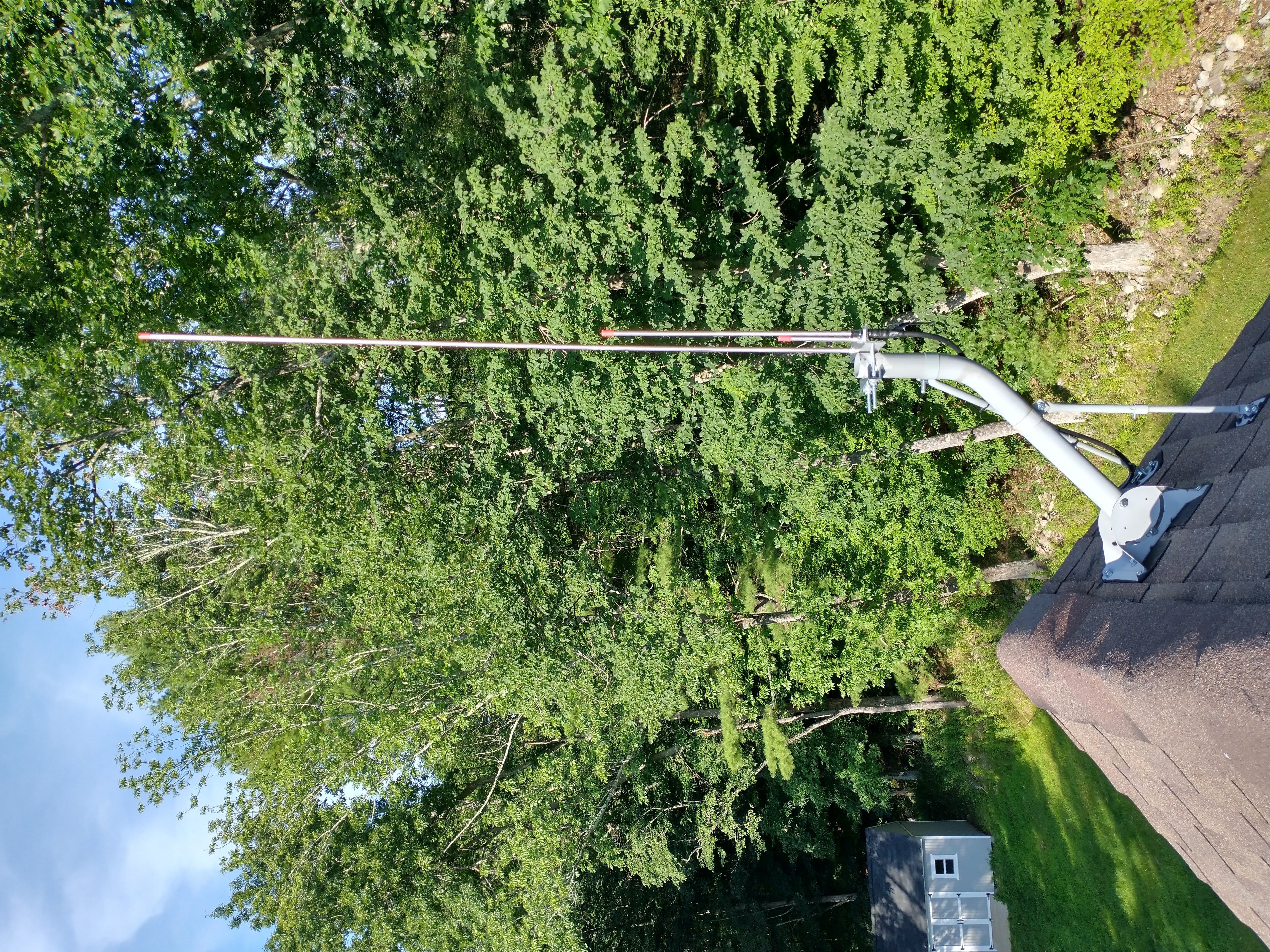
Open-Stub J-Pole Analysis
Once down from the roof, I began my analysis. There are some free simulators out there that use the NEC7 on one end of the (electromagnetic?) spectrum. At the other end are the enterprise-level RF design tools such as Microwave Office8, ADS9, and Ansys10. Did you know that it doesn't take a full RF design software license to get a good idea of antenna performance? Even just an SI/PI analysis suite such as Cadence Sigrity can get us what we need. The Sigrity 3DEM license along with 3D Workbench 11 provides a perfect environment to quickly model arbitrary 3-D geometry and determine parameters such as resonant frequency, VSWR / S11 , and far-field radiation patterns. It may not automatically give detailed results such as efficiency or directivity but it's plenty to give an idea of behavior and allows the designer an opportunity to modify a design to meet any project requirements.
Figure 2. OSJ model in Cadence 3D Workbench.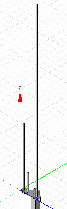
Figure 3. OSJ model, UHF connector detail.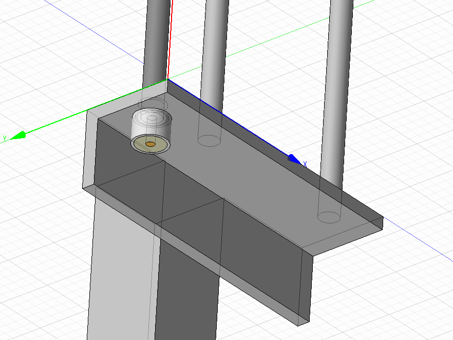
The antenna was simulated as if mounted to a 100" insulated pole. The range of 100 MHz to 500 MHz was selected in order to ascertain behavior in both the 2m and 70cm bands. The UHF connector12 was originally modeled, but I realized that I didn't have accurate dimensions of the SO-239 stud or coupling nut, and I wouldn't want to introduce reflections which are not representative of the antenna structure itself.
Results
The results confirmed exactly what some reviews have stated: performance is slightly worse in the 70cm band. S11 (converted to VSWR ) does indicate this, with a best-case SWR of 1.2 in the 70cm band, and 1.1 in the 2m band.
Figure 4. OSJ return loss (S11).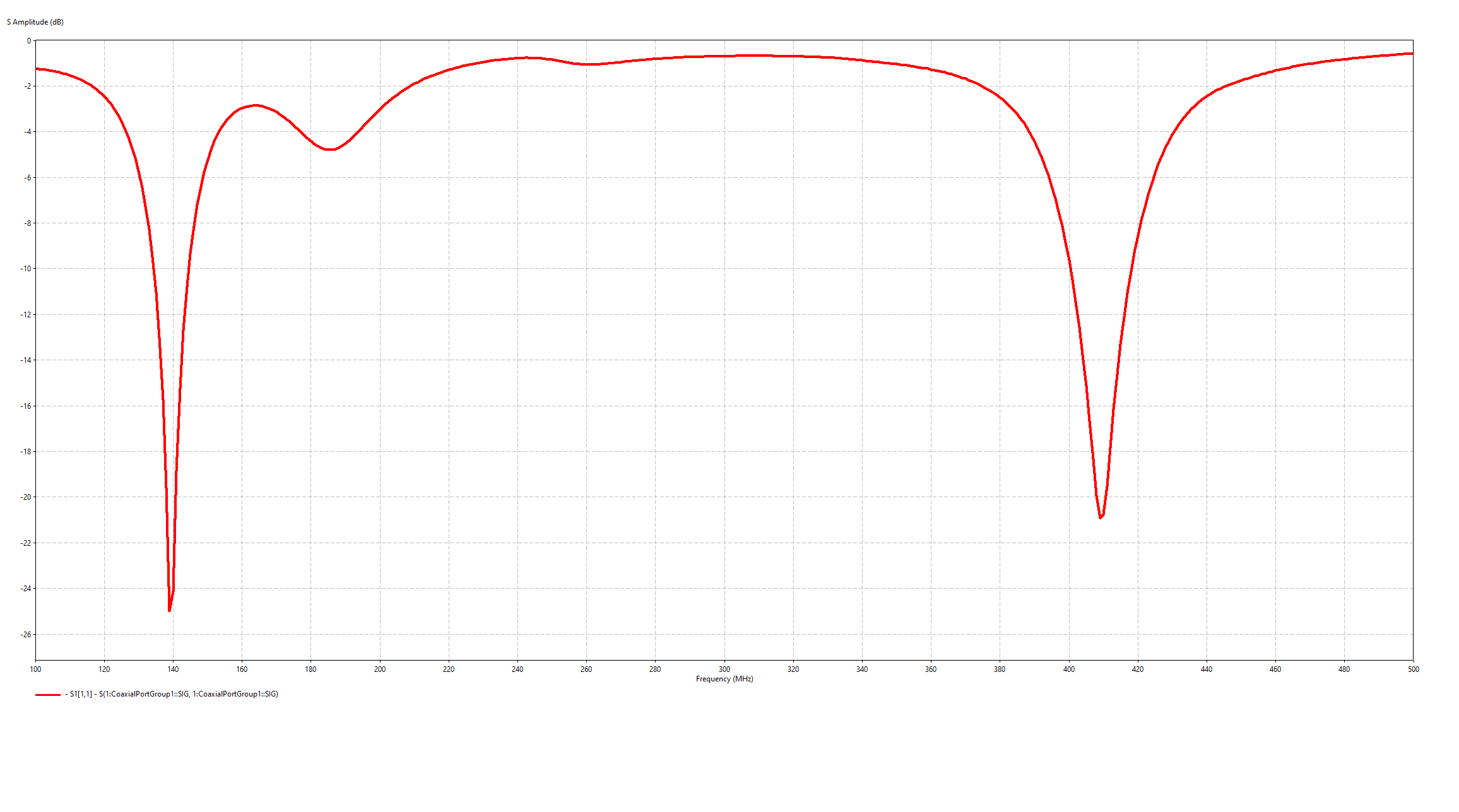
Figure 5. OSJ VSWR.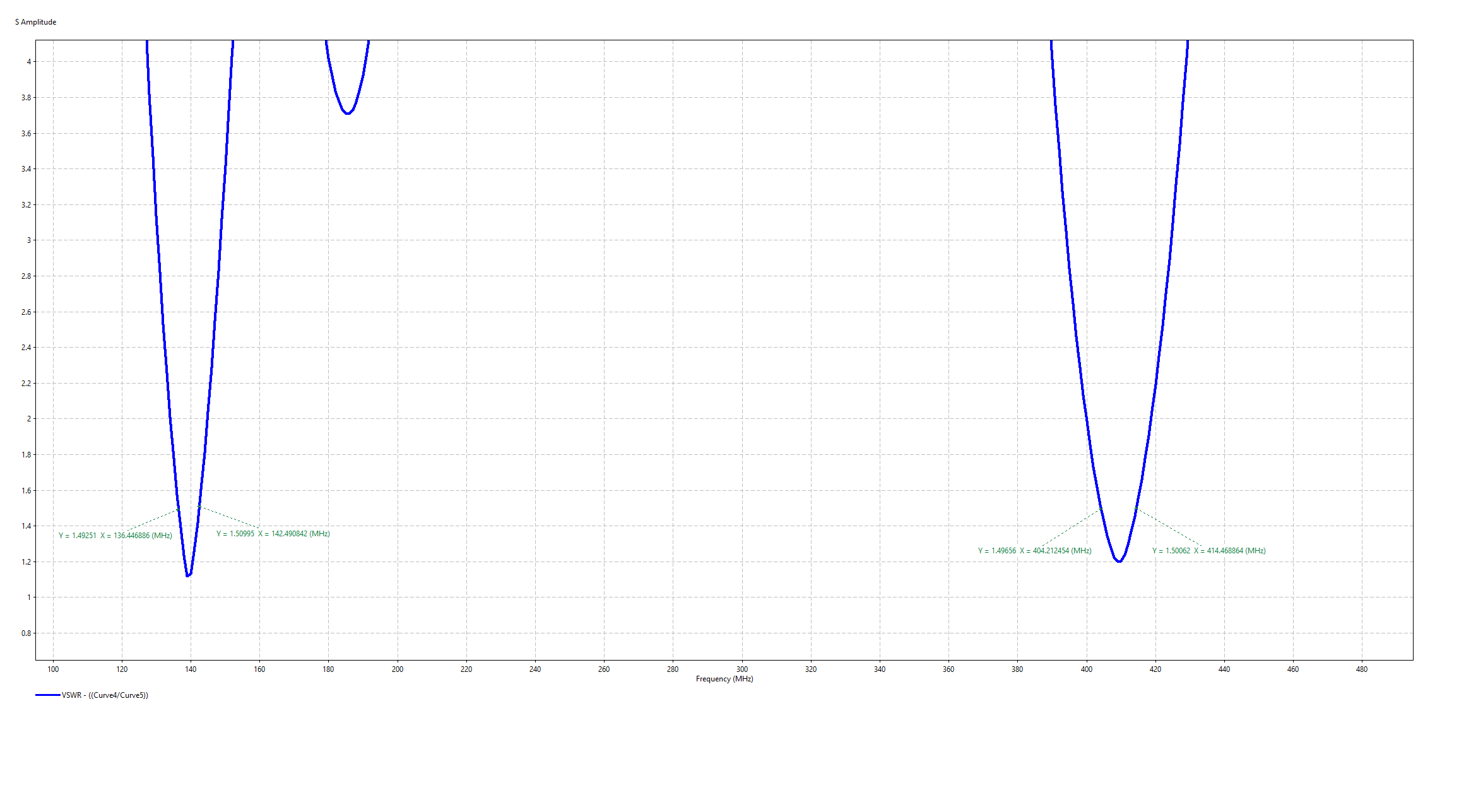
One of the most interesting things about this analysis is that the center frequency for both bands is quite a bit different from what is reported. The Arrow SWR chart13 shows the 2m band coverage from 142-150 MHz and the 70cm from 430-453 MHz. Our analysis shows the 2m band covering 136-142 MHz and the 70cm band covering 404-414 MHz - both lower than expected. This should be confirmed with an antenna analyzer, though one is not currently available to make the measurement. Interesting to note - I'm not the first person to notice these discrepancies when simulating against the instruction manual's dimensions14. I did make a point to measure the antenna and each element was within 1/4" of the stated dimensions. That made me even more eager to get an analyzer on it to test its actual response. At that point, I tweaked the model to match measurements and ensure the feed point is modeled correctly. For now though - the goal is simply to determine propagation directionality which I'll analyze in the next section.
Far Field Propagation
Finally, we arrive at my ultimate goal - determining whether or not propagation is truly omni-directional ! The fastest way to check this out is to look at the far-field propagation plots. For reference, Fig. 6 shows the orientation of the antenna in relation to the axes. We are specifically looking for any directivity at all in the antenna. All plots will indicate the frequency of interest, and every plot was generated with a 1V source (13 dBm) and field strength is simulated at a distance of 3m.
Figure 6. Antenna orientation.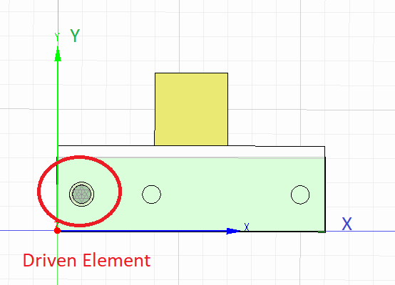
First, I'll present an isometric view of the propagation pattern. It's important to note that the units are given in mV/m for the 3D plots, but dBuV/m for the 2D plots to follow. This makes the magnitude of variation seem greater in the 3D plots, but we can probe for specific values on the 2D plots. (Click any of the propagation plots for a larger view).
Figure 7. Far field, 139 MHz, isometric view.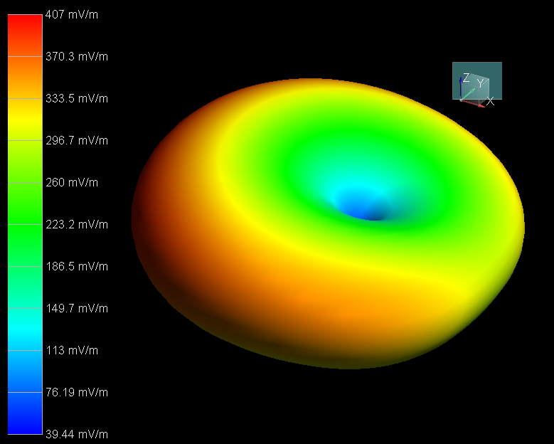
The isometric view is the first indication that we aren't looking at purely omni-directional propagation. As fun as the 3D views are to look at, we can get the specific difference with a 2D plot.
Figure 7. Far field, 139 MHz, top-down cut on the XY-plane (Z=0).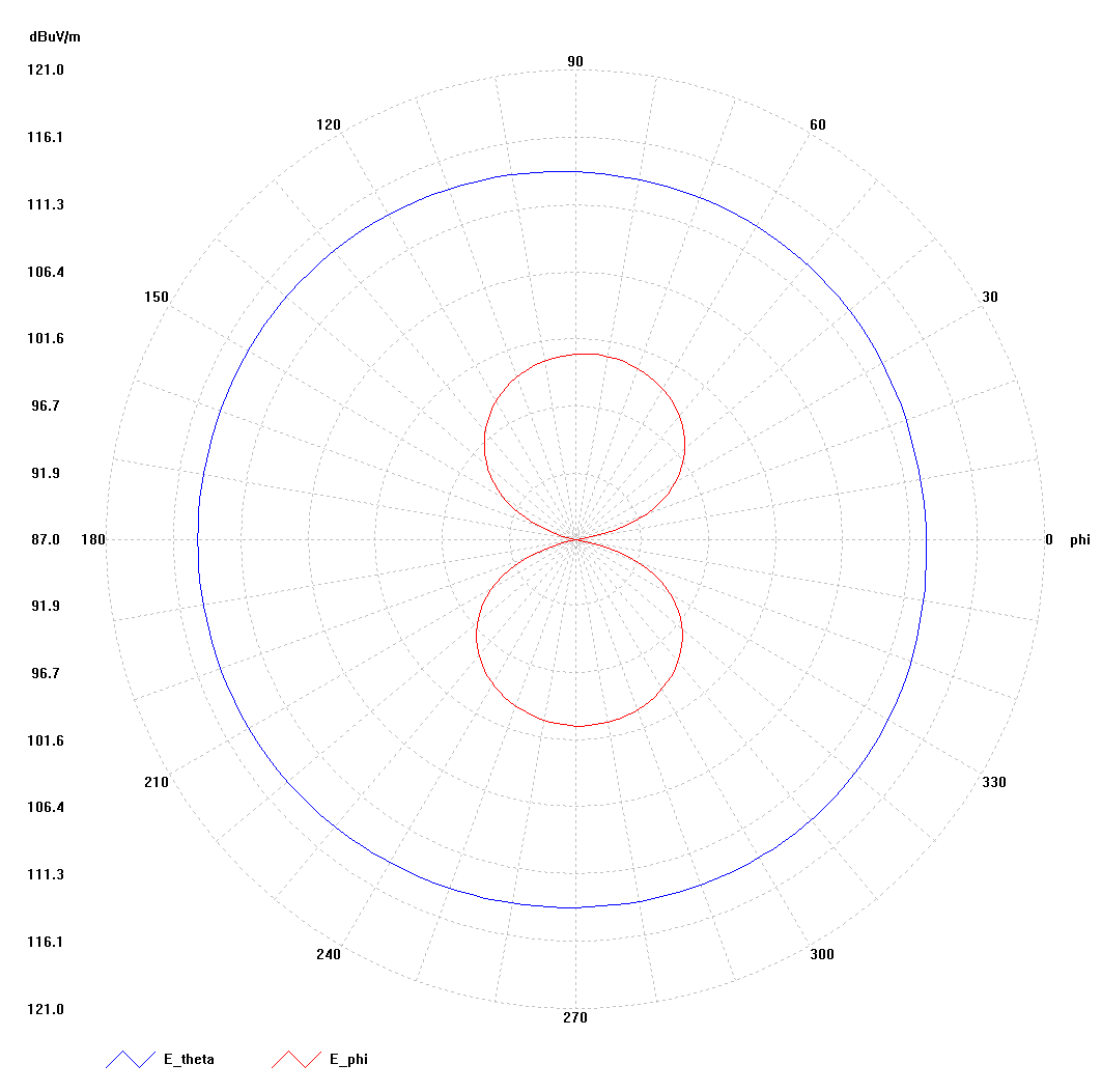
As it turns out, there is a minor difference in propagation depending on the angle ɸ. The maximum value at ɸ=180deg is 114.4 dBuV/m, and the minimum value at ɸ=0deg is 112.4 dBuV/m. It would be nice to represent this as a dBi difference. Using an online calculator15 (they're always right of course!) we can determine the gain of the antenna in dBi. In this case, we see a gain of 6.2 dBi in the forward direction and 4.2 dBi in the backward direction for a 2 dB front-to-back ratio. Coincidentally, this was my guess while on the roof and was the orientation I used while mounting the antenna. This may not be extremely significant but it's worth knowing while mounting the antenna.
Surprisingly, there's even more directivity at 70cm, although that won't matter for me and my 2m-only radio.
Figure 8. Far field, 410 MHz, top-down view.
The bottom-line answer to my original question is that if you really need to squeak out every last bit of gain in a certain direction, then you'd be better off mounting the J-pole with the driven element closer to that desired direction.
One last thing - if anyone is looking at more simulations or measurements, here's the Touchstone16 file for this simulation which can be downloaded and compared. Let me know if you use it!
What about that QSO?
As of publication my friend and I have yet to close the link on a successful exchange. This could be due to any number of factors, but I was able to make contact with another ham via a repeater located 30 miles from my QTH2, so the reasonable assumption is that the antenna system on my roof is operating well.

NanoVNA - Used to Measure Antennas
In this post, we look at antenna characteristics. This instrument is a very low-cost way to make measurements of your antennas (among other things). It's not perfect and has relatively low performance compared to 'real' VNAs, but it costs about 1/100th of anything else!
PCB antenna
While analysis of ham radio antennas is an interesting pursuit, it caused me to stop and consider more practical applications of this software. One thing that really struck me was the huge rise in IoT devices using Bluetooth , Wi-Fi , NFC , and many other wireless communication protocols. How can a designer be assured their antenna will work as required? Sure, copying dimensions from datasheets or other resources might be adequate but for optimal performance on the first fab run, a simulation would be very helpful. As an example, I've chosen a common antenna design and show how quick and easy it is to simulate and validate prior to fabrication.
Antenna Selection
Cypress has an excellent document17 describing antenna and RF design. Even better, they have links to PCB designs of a few antennas which can be adapted to a designer's board. I chose to import and simulate their MIFA (Meandered Inverted-F Antenna).
Figure 9. MIFA 3D view.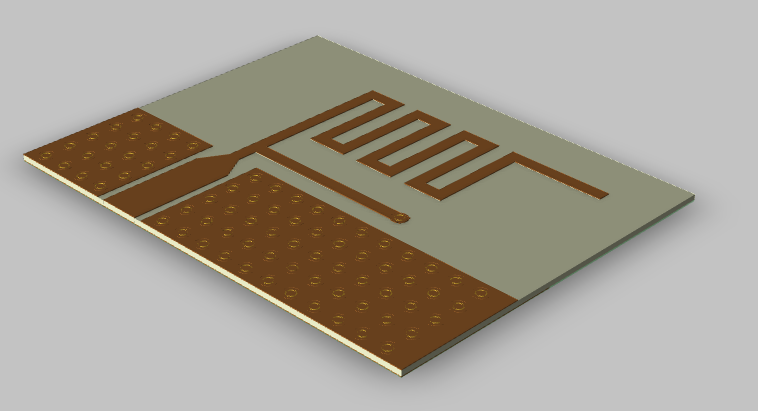
Prior to beginning the simulation we must determine the PCB stackup and materials used. Fortunately the linked design files include a fabrication drawing which indicates a finished PCB thickness of 62mils. The material is listed as generic FR-4, so we'll use one of the most common FR-4 materials available: Isola 370HR18.
Next, the board design must be imported into the simulation tool of choice. In this case, I'll bring the .brd file into PowerSI 3D-EM in order to tweak the stackup. From there, we'll save it as a .spd and bring that into 3D Workbench .
Figure 10. MIFA 3D view with Lumped Port in 3D Workbench.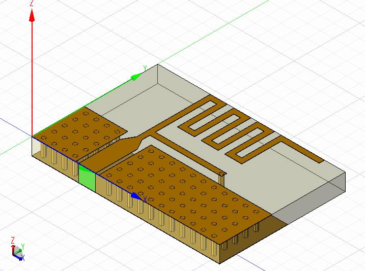
Initial Simulation
The first simulation shows that this board must have been designed specifically for manual adjustment given the resonant frequency is 2.1 GHz (see Fig. 11 below). We could raise the resonant frequency by either thinning the board or shortening the tail of the antenna. Since the fabrication drawing specifies that this is to be a 62mil board, we can adjust the tail and see how performance changes.
Figure 11. MIFA S11, unmodified.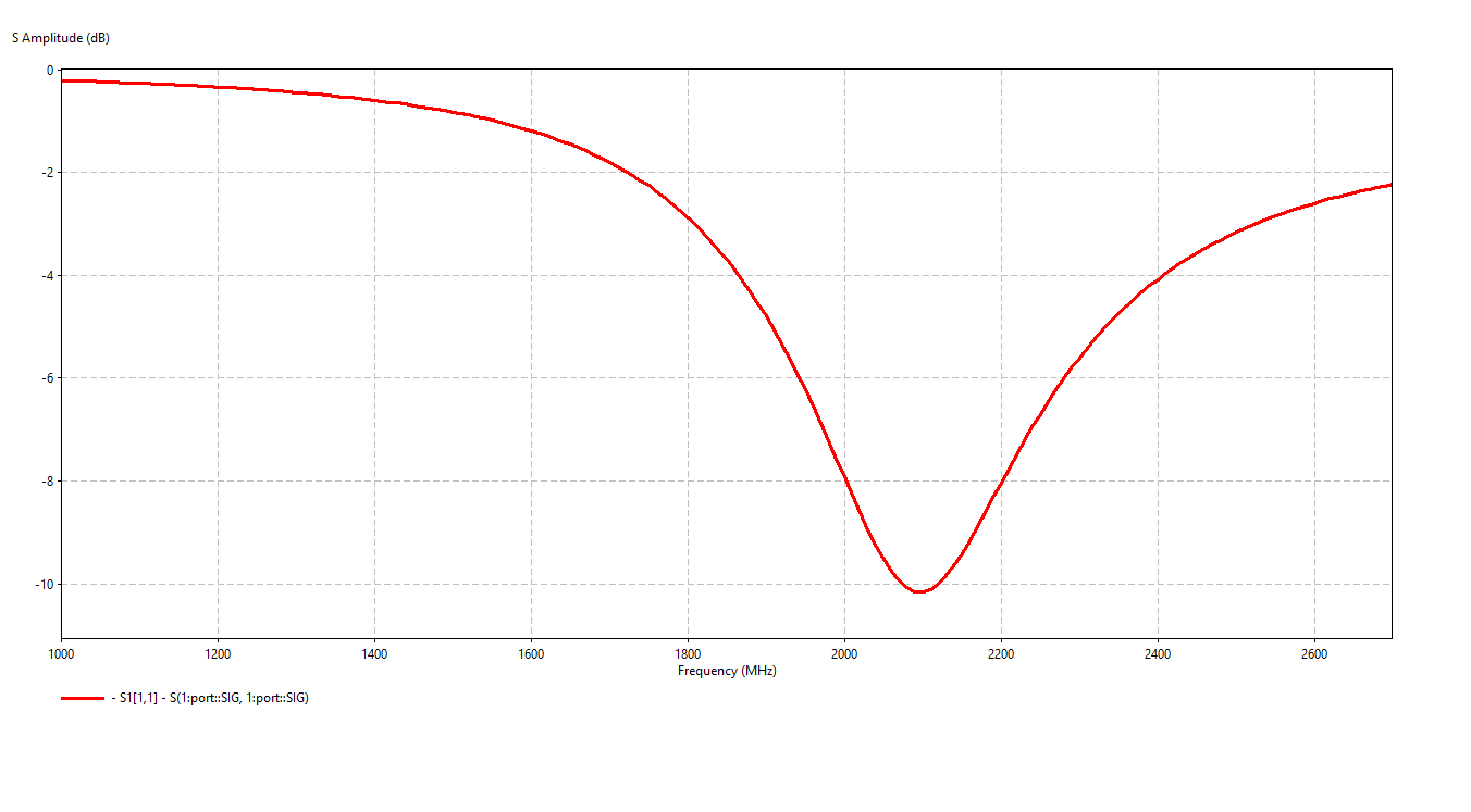
The Cypress document includes some recommended tail dimensions based on the board thickness in its Table 3. Using that as a start, we set the leg to 115mils and see where that gets us. We can quickly iterate and determine that setting the leg length to 45mils centers the antenna resonance at exactly 2.4GHz.
Figure 12. MIFA 3D view after modification.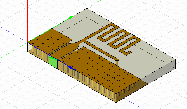
Figure 13. MIFA S11, modified.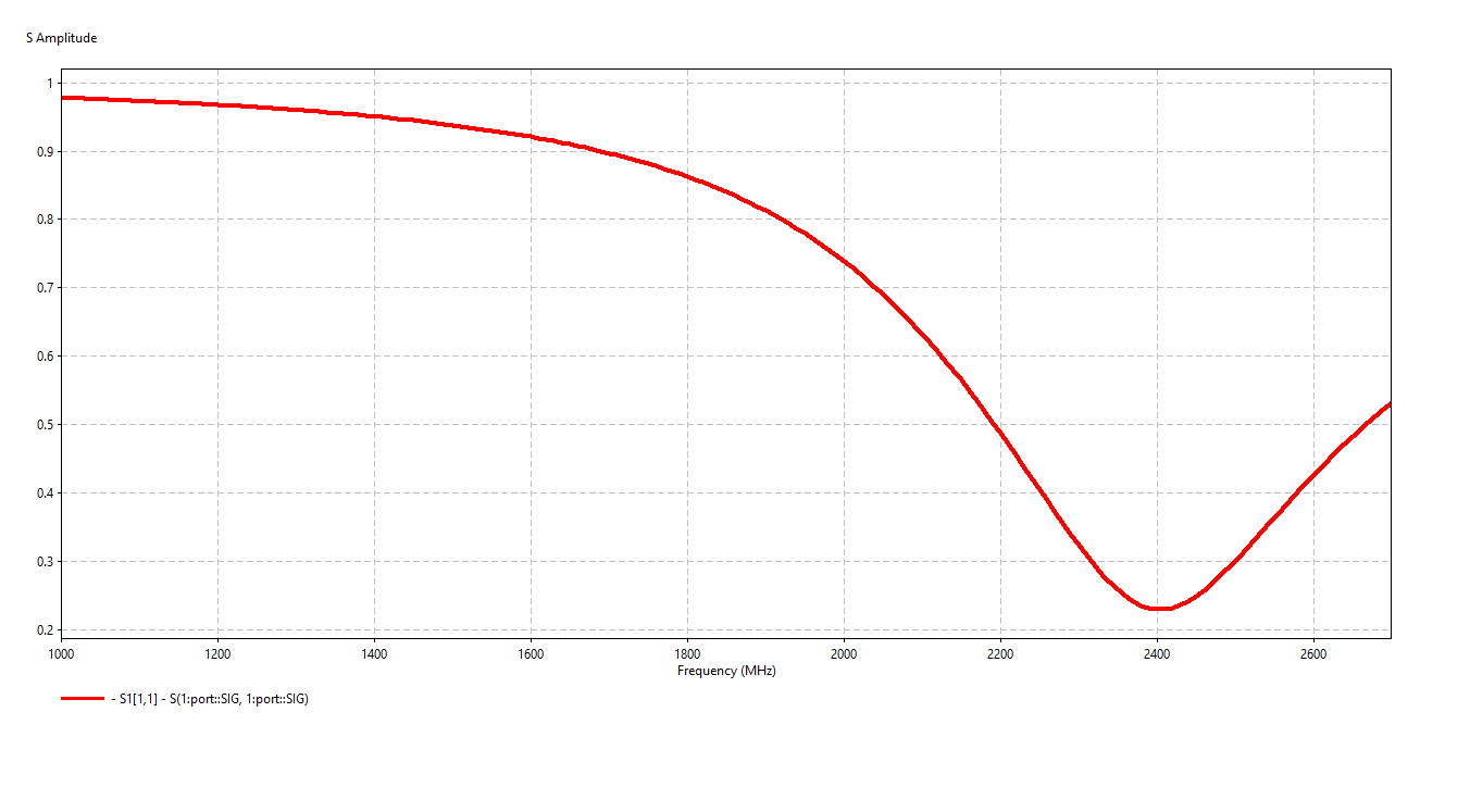
Impedance Match
Unfortunately, a quick check of the Smith chart19 shows an issue. The impedance match at resonance is right at 75Ω rather than the expected 50Ω. If we need to hook this up to our 50Ω transmission lines, we'll need to add a matching circuit.
Figure 14. MIFA S11, modified, Smith chart.
Fortunately, there's an excellent Smith Chart matching tool available for free download! The Iowa Hills Smith Chart tool20 can be used to quickly find the impedance match circuit. Starting with the input impedance of 75Ω, we can add a shunt inductor then a series capacitor.
Figure 15. MIFA Smith chart impedance match calculation.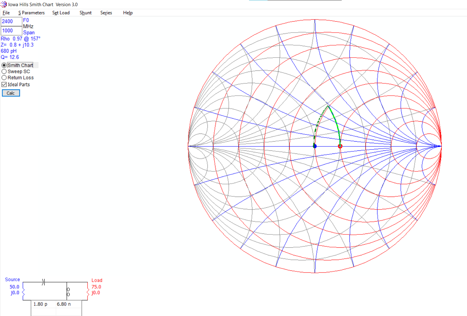
In reality, we would want to account for the parasitics of the components, but this will get us close enough for an estimate. We can use the SystemSI tool to add a few discrete components and extract an S-parameter response of the entire system.
Figure 16. MIFA impedance match circuit.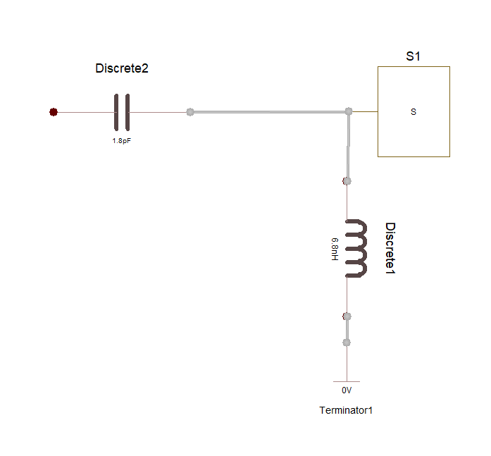
We can see that after impedance matching, we've significantly reduced the reflected energy seen by the transmitter. There has been a bit of a shift in frequency, but given the improved return loss the bandwidth of the antenna now ranges from nearly 2.25 GHz to 2.55 GHz. This is also clearly seen in the Smith chart.
Figure 17. MIFA S11 before and after impedance matching.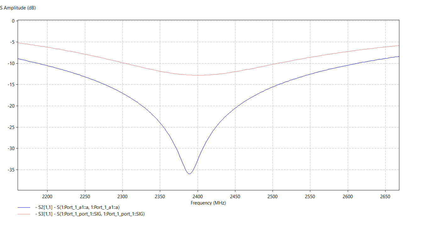
Figure 18. MIFA S11 (Smith chart) before and after impedance matching.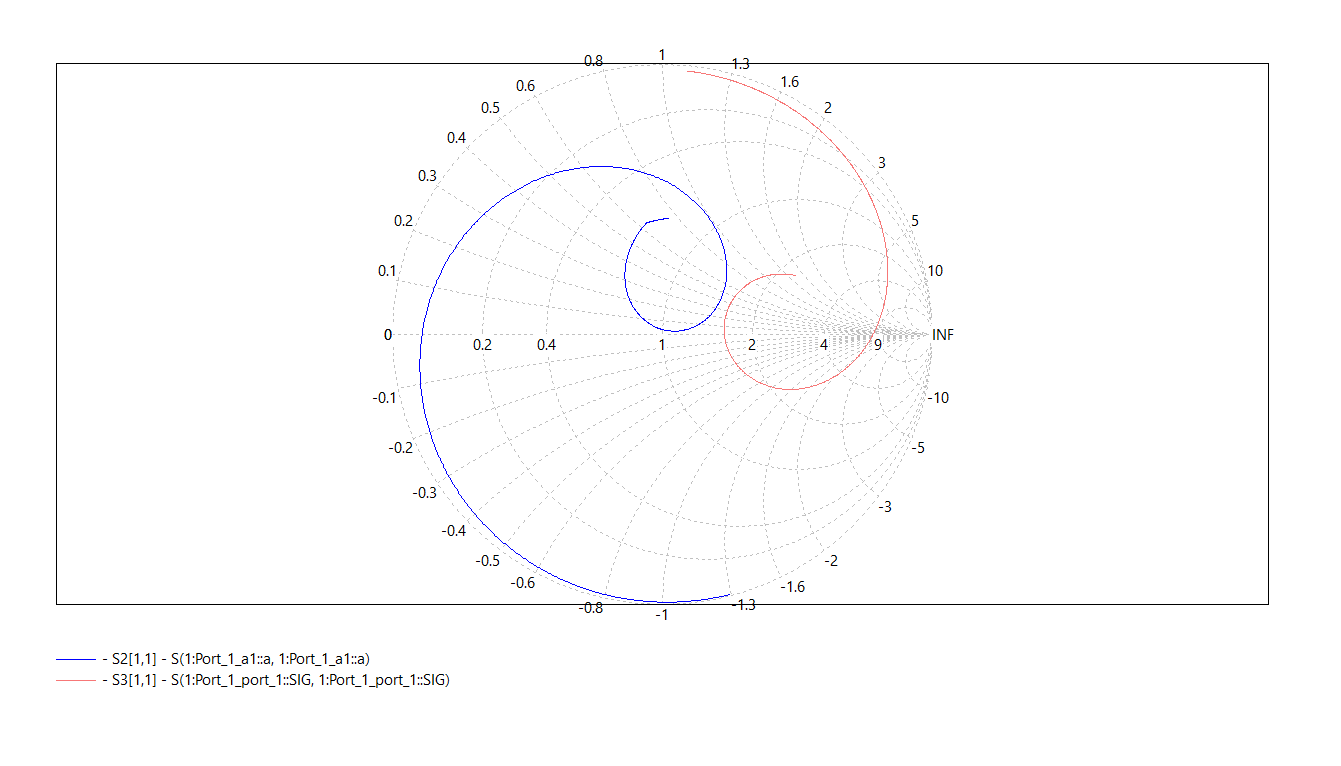
Far-Field Propagation
The last thing we can do with the PCB antenna here is verify the far-field propagation. If we know this device will be oriented in a certain way, we can ensure propagation will be optimized for that application. In order to provide a reference for plot axes, the orientation is depicted below.
Figure 19. MIFA far-field orientation.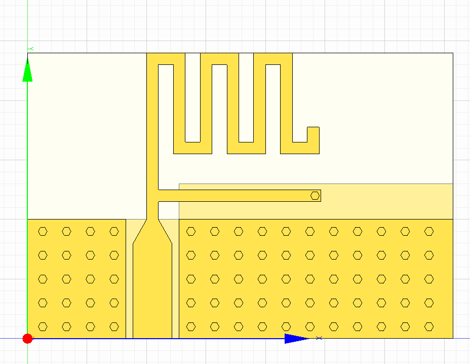
We can see from Fig. 20 that the far-field propagation looks pretty good, extending strongest in the +x and -x directions.
Figure 20. MIFA far-field at 2.4 GHz, X-Y Plane.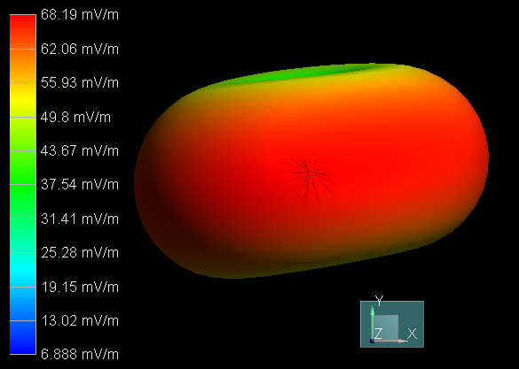
Checking it out in a 2-D plot reveals a reasonably large area of attenuation in the direction of the PCB, so for best results we want to make sure to orient the PCB itself away from other receivers.
Figure 21. MIFA far-field at 2.4 GHz, X-Y Plane (2-D plot).
Conclusion
This article has been an exciting exploration of both standalone and PCB-based antennas. The key takeaway is that there's no requirement for a dedicated RF engineer and extremely costly RF analysis software in order to verify and optimize the design of PCB-based antennas. Rather, the designer can use more common signal integrity software to quickly determine the behavior of the antenna and make small adjustments to meet requirements.
Given the amount of variability described in the Cypress documentation due to effects such as plastic enclosures, the designer could even use these tools to model environmental materials and determine any potential frequency shifts.
This would improve time-to-market and reduce development costs compared to a full, comprehensive analysis. At the same time, these small steps will increase performance in comparison to using basic application note rules and suggestions.
Future Work
Despite peer corroboration that the Arrow OSJ antenna simulations often indicate a frequency lower than measured, I strongly dislike the possibility of discrepancy. I plan to follow up with two specific points of investigation:
- A precise measurement of the antenna itself. This could prove difficult now that it's installed and weather-proofed, since the 100 ft of RG-8X would attenuate much of the returned energy.
- Optimization of the simulated feed point and improvement of the antenna simulation model to ensure simulation matches antenna measurements.
Footnotes
Here's more info than you could ever want from the ITU regarding attenuation in vegetation: Recommendation ITU-R P.833-9 [PDF]
The ARRL provides ample guidance for electromagnetic safety including links to an RF Safety Calculator.
Low-resolution antenna propagation plot given by Arrow Antennas for the OSJ in 2m.
Arrow Antenna's SWR chart:
Dr. Milazzo (KP4MD) also indicates frequency results lower than specifications when simulating the Arrow OSJ antenna.
A Touchstone file is used for viewing N-port S-parameter data. A free program for viewing and simulating is available: http://qucs.sourceforge.net/
More info on Touchstone files: https://en.wikipedia.org/wiki/Touchstone_file
See document number 001-91445: https://www.cypress.com/file/136236/download
https://www.isola-group.com/products/all-printed-circuit-materials/370hr/
Note that 370HR lists its generic Dk/Df as 4.04/0.021 which is sufficient for this simulation. Greater detail would demand knowledge of the exact weave/resin style with more specific Dk/Df values.
The Smith chart is an excellent tool for viewing impedance match over frequency.
The Smith chart tool can be downloaded here: http://www.iowahills.com/8DownloadPage.html
There's a wealth of information on how to use the tool and about Smith charts in general here: http://www.iowahills.com/9SmithChartPage.htmlv
Table of Contents
Related Engineering Insights
Parallel Plate Capacitor Equation - Simulated
The Question
A recent homework problem had us derive the parallel plate …
Using PSPICE Components in LTspice
A recent post on the PCEA Discord server requested a bit of assistance using …
Webinar Recording: DDR5 Post-Layout Verification: Find and Fix Causes of Failure
I recently presented (another) webinar with EMA Design Automation to discuss …
